Warning

The content of the following page is based on the SPHN RDF schema version 2021.2.

Use Python and R with RDF data

Note

To find out more watch the How to use Python and R with RDF data Training

The examples used in this page are based on the mock-data introduced in the “Graphical exploration of data with GraphDB” section (see mock-data description and loading instructions). The SPARQL queries employed in these examples build upon the previously introduced query examples (learn more about Query data with SPARQL).

The instructions presented in this page have been integrated in a notebook.

Target Audience

This document is mainly intended for researchers and RDF experts who are interested in analysis their data through other means than using a triplestore. It showcases how RDF graphs can be queries and ‘manipulated’ with two programmating languages: R and Python.

Overview

This section tackles different languages and development environments which are summarized in Table 1. For installation guides please refer to the documentation provided in the following links:

Table 1: Overview of the employed languages, development environments, and graph database.
Language	Development environment	Graph database
Python	Jupyter	GraphDB
R	R Studio	GraphDB

Loading data from GraphDB in Python and R

Step 1: Handle dependencies

Python

In order to access the RDF data loaded in GraphDB from Python, the SPARQL Endpoint interface to Python ‘SPARQLWrapper’ is employed. The following code example shows how to install a pip package in the current Jupyter kernel and import the module in Python:

import sys
!{sys.executable} -m pip install --upgrade SPARQLWrapper

from SPARQLWrapper import SPARQLWrapper, JSON

R

In order to access the RDF data loaded in GraphDB from R, the SPARQL package is employed. The following code example shows how to install a package in R studio and import the library in R:

install.packages("SPARQL")

library(SPARQL)

Step 2: Setup a connection to a SPARQL endpoint

The following examples show how to setup a connection to a GraphDB SPARQL endpoint running on localhost.

Python

A connection in Python can be setup by creating an instance of the SPARQLWrapper class, as demonstrated in the following example:

#  Connect to GraphDB running on localhost
host_name = "localhost"
port = 7200
project_name = "sphn_demo"
sparql = SPARQLWrapper("http://" + host_name + ":" + str(port) + "/repositories/" + project_name)

An example of the SPARQL endpoint URL is shown in Figure 1. One can see that it is composed of the Graphdb server’s URL (i.e., localhost), the default server port (i.e., 7200) and the repository ID (i.e., sphn_demo).

Figure 1: Endpoint of a SPARQL connection in Python.

R

A connection in R can be setup as follows:

# Setup a connection to GraphDB running on localhost
host_name = "localhost"
port = 7200
project_name = "sphn_demo"

endpoint <- paste0("http://", host_name, ":", port, "/repositories/", project_name)

prefixes <- c('sphn-resource','<https://biomedit.ch/rdf/sphn-resource/>')

The endpoint defined in R is exactly the same as the one defined in Python, as shown in Figure 2:

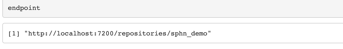
Figure 2: Endpoint of a SPARQL connection in R.

Step 3: Define the query

In the following examples, a query for retrieving patients annotated to be allergic to Pulse Vegetable is used. The query is defined as a string variable.

Python

In Python, a query can be defined as a multi-line string using the """ syntax, as demonstrated in the following example:

# Query for patients allergic to Pulse Vegetable
query_string = """
PREFIX rdf:<http://www.w3.org/1999/02/22-rdf-syntax-ns#>
PREFIX rdfs:<http://www.w3.org/2000/01/rdf-schema#>
PREFIX sphn:<https://biomedit.ch/rdf/sphn-ontology/sphn#>
PREFIX resource:<https://biomedit.ch/rdf/sphn-resource/>
PREFIX xsd:<http://www.w3.org/2001/XMLSchema#>
PREFIX snomed: <http://snomed.info/id/>

SELECT DISTINCT ?patient
WHERE {
    ?patient a sphn:SubjectPseudoIdentifier .
    ?allergy_episode a sphn:AllergyEpisode .
    ?substance a sphn:Substance .

    ?allergy_episode sphn:hasSubjectPseudoIdentifier ?patient .
    ?allergy_episode sphn:hasSubstance ?substance .
    ?substance sphn:hasSubstanceCode ?substance_code .

    ?substance_code a ?pulse_veg_and_descendants .
    ?pulse_veg_and_descendants rdfs:subClassOf* snomed:227313005 .
}
"""

R

In R, a query can be defined as a string by putting it between either single or double quotation marks (i.e., '...' or "..." ), as demonstrated in the following example:

# Query for patients allergic to Pulse Vegetable
query_string = '
PREFIX rdf:<http://www.w3.org/1999/02/22-rdf-syntax-ns#>
PREFIX rdfs:<http://www.w3.org/2000/01/rdf-schema#>
PREFIX sphn:<https://biomedit.ch/rdf/sphn-ontology/sphn#>
PREFIX resource:<https://biomedit.ch/rdf/sphn-resource/>
PREFIX xsd:<http://www.w3.org/2001/XMLSchema#>
PREFIX snomed: <http://snomed.info/id/>

SELECT DISTINCT ?patient
WHERE {
    ?patient a sphn:SubjectPseudoIdentifier .
    ?allergy_episode a sphn:AllergyEpisode .
    ?substance a sphn:Substance .

    ?allergy_episode sphn:hasSubjectPseudoIdentifier ?patient .
    ?allergy_episode sphn:hasSubstance ?substance .
    ?substance sphn:hasSubstanceCode ?substance_code .

    ?substance_code a ?pulse_veg_and_descendants .
    ?pulse_veg_and_descendants rdfs:subClassOf* snomed:227313005 .
}
'

Step 4: Run the query and retrieve results

Python

In Python, before running the query, the return format is set to JSON in order to generate a Python dictionary (for alternatives see here). Running a query and retrieving results can then be done as follows (note the use of the method chaining where multiple methods are called on a single object in a sequence):

# load the query and set the return format
sparql.setQuery(query_string)
sparql.setReturnFormat(JSON)

# run the query and retrieve results
results = ( sparql
           .query()
           .convert()
          )

The results can then be accessed by iterating over the retrieved Python dictionary, and indexing value with name of the retrieved SPARQL variable of interest (e.g., patient index for the ?patient variable; see Figure 3 for an excerpt of the results).

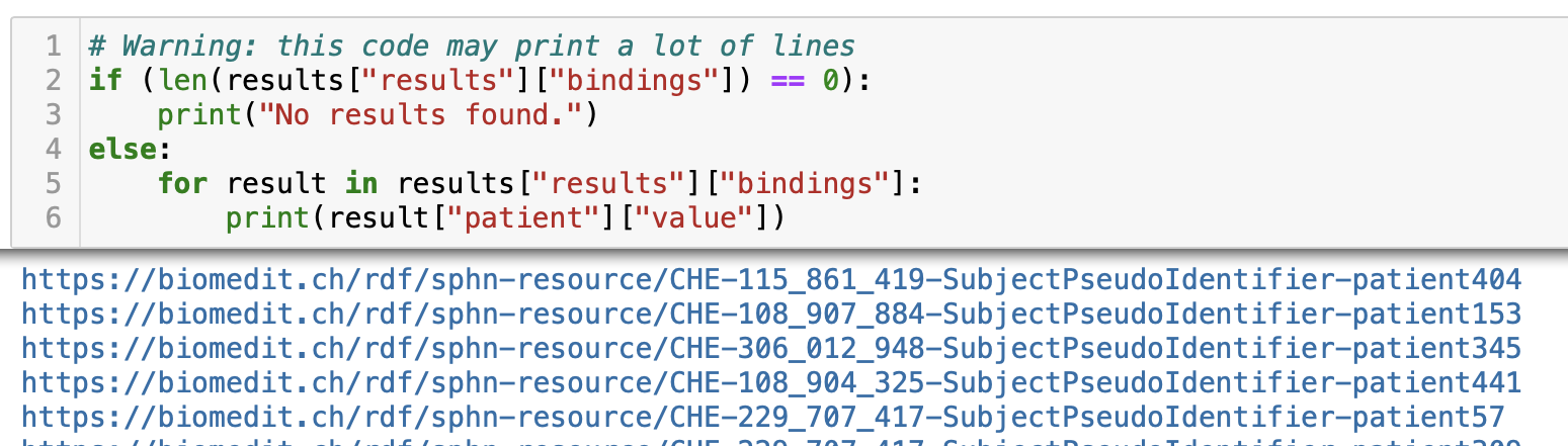
Excerpt of retrieved results when running the query for Patients allergic to Peanuts on the mock-data (Note: GraphDB SPARQL endpoint running on localhost).

Figure 3: Excerpt of results obtained when running the query about Patients allergic to, here specifically, Peanuts, on the mock-data (Note: The GraphDB SPARQL endpoint is running on localhost).

R

In R, a query can be run by calling the SPARQL method and passing in the parameters. In addition to the endpoint and query_string parameters defined in previous steps, one can also pass in the prefixes to shorten the IRIs. The results can then be retrieved as follows:

# run query and retrieve results
query_results <- SPARQL(endpoint, query_string, ns=prefixes)

The results are retrieved as a data frame, containing a column for each selected variable. Note that in the special case of selecting one variable only, the resulting data frame is somewhat different (see next section on how to deal with this).

Combining results from different queries

The results of the following two queries are going to be combined:

Query for patients allergic to Pulse Vegetable
Query for patients with measurements of Leukocytes in Blood

To that end, the results will be converted to a dataframe. While not a mandatory step, this often makes it easier to combine results from different queries.

Converting the results to a dataframe

Note

This section contains introductory material on dataframes in Python and R. Those already familiar with this topic can skip / scroll over to the next section.

Python

An example of a dataframe in Python is shown in Figure 4.

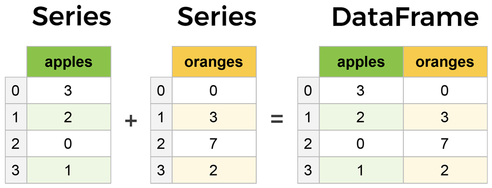
Figure 4: Example of a dataframe in Python.

Converting the results to a dataframe in Python can be done as follows (see Figure 5 for an excerpt of the results):

# simple conversion of 'result' dictionary to a pandas dataframe
# (for a more advanced conversion see, e.g., https://github.com/RDFLib/sparqlwrapper/issues/125)
import pandas as pd

df_pulse_vegetable = pd.DataFrame(columns=['patient'])

for result in results["results"]["bindings"]:
        df_pulse_vegetable = df_pulse_vegetable.append({
            'patient': result["patient"]["value"]
        }, ignore_index=True)

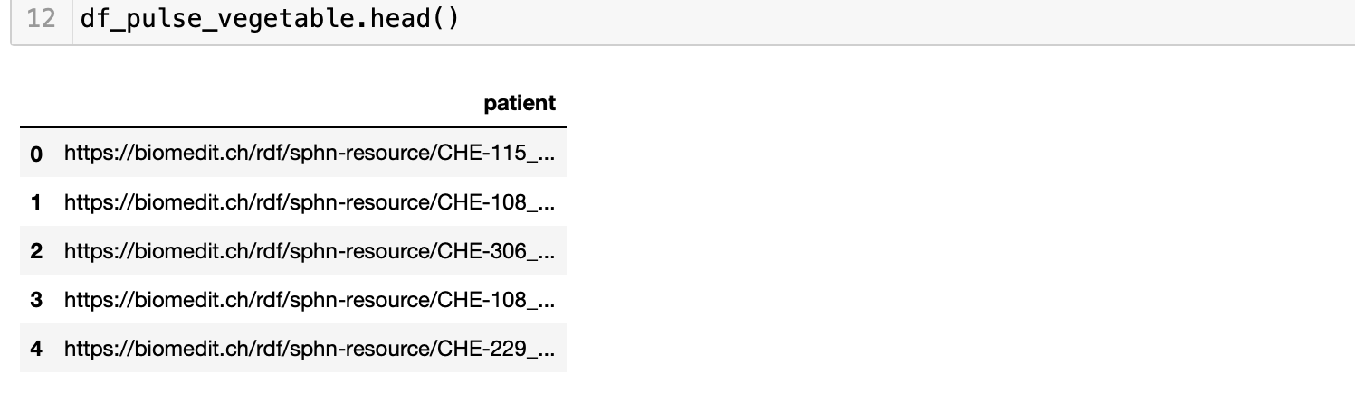
Excerpt of the results following the conversion to a dataframe in Python.

Figure 5: Excerpt of the results transformed into a dataframe in Python.

R

While dataframes are native to R, in some cases (e.g. when selecting one variable only) the results are in a somewhat inconvenient form. A more convenient form is the so called tidy data (see Figure 6)

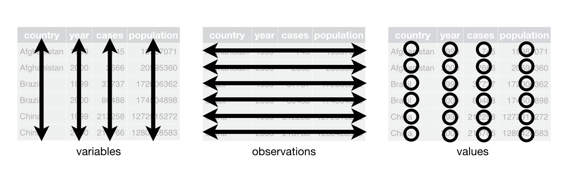
Figure 6: Tidy data.

One can achieve this form by applying the following transformation (see Figure 7 for an excerpt of the results):

# convert the results to a dataframe
df_pulse_vegetable <- as.data.frame(apply(query_results$results, 2, as.character))

colnames(df_pulse_vegetable) <- c('patient')

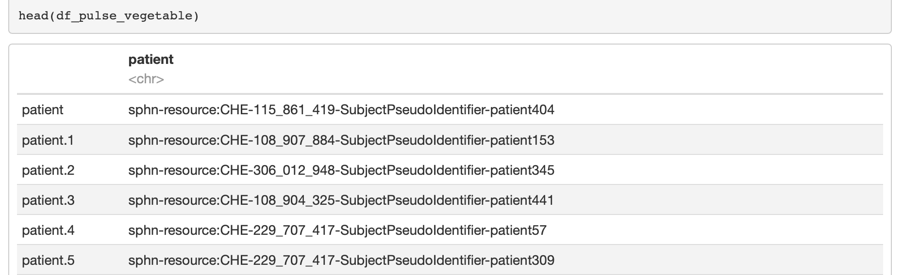
Figure 7: Excerpt of the results in a ‘tidy’ R dataframe.

Dealing with various datatypes (datetime, numeric, etc.)

Here, in order to demonstrate how to deal with various datatypes the existing Query for Patient with measurements of Leukocytes in Blood is modified to include:

Lab result analysis datetime

Lab result value

Lab result unit

Python

The modified query is run in Python as follows:

# Modified query for Patient with measurements of Leukocytes in Blood
query_string = """
PREFIX rdf:<http://www.w3.org/1999/02/22-rdf-syntax-ns#>
PREFIX rdfs:<http://www.w3.org/2000/01/rdf-schema#>
PREFIX sphn:<https://biomedit.ch/rdf/sphn-ontology/sphn#>
PREFIX resource:<https://biomedit.ch/rdf/sphn-resource/>
PREFIX xsd:<http://www.w3.org/2001/XMLSchema#>
PREFIX loinc: <https://loinc.org/rdf/>
PREFIX sphn-loinc: <https://biomedit.ch/rdf/sphn-resource/loinc/>

SELECT DISTINCT ?patient ?lab_res_analysis_datetime ?lab_res_value ?lab_res_unit
WHERE {
    ?patient a sphn:SubjectPseudoIdentifier .
    ?lab_res a sphn:LabResult .

    ?lab_res sphn:hasSubjectPseudoIdentifier ?patient .
    ?lab_res sphn:hasLabResultLabTestCode ?test_code .

    ?test_code rdf:type ?loinc .
    ?loinc sphn-loinc:hasComponent "Leukocytes" .
    ?loinc sphn-loinc:hasSystem "Bld" .

    ?lab_res sphn:hasLabResultAnalysisDateTime ?lab_res_analysis_datetime .
    ?lab_res sphn:hasLabResultValue ?lab_res_value .
    ?lab_res sphn:hasLabResultUnit ?lab_res_unit.
}
"""

#load the query and set the return format
sparql.setQuery(query_string)
sparql.setReturnFormat(JSON)

# run the query and retrieve results
results = ( sparql
           .query()
           .convert()
          )

The following code blocks demonstrate how to get datetimes and numeric values from the retrieved string representations (see Figure 8 for an excerpt of the results):

# simple conversion of 'result' dict to a pandas dataframe
# (for a more advanced conversion see, e.g., https://github.com/RDFLib/sparqlwrapper/issues/125)
df_leukocytes_meas = pd.DataFrame(columns=['patient', 'lab_res_analysis_datetime', 'lab_res_value'])

for result in results["results"]["bindings"]:
        df_leukocytes_meas = df_leukocytes_meas.append({
            'patient': result["patient"]["value"],
            # convert the 'lab_res_analysis_datetime' to pandas datetime
            'lab_res_analysis_datetime': pd.to_datetime(result["lab_res_analysis_datetime"]["value"]),
            # convert the 'lab_res_value' to numeric
            'lab_res_value': pd.to_numeric(result["lab_res_value"]["value"]),
            # also add a column for the unit(for the mock-data)
            'lab_res_unit': result["lab_res_unit"]["value"]
        }, ignore_index=True)

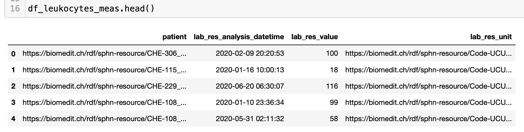
Figure 8: Excerpt of the results following the datatype conversion in Python.

R

The modified query is run in R similarly as in Python, albeit with the following difference:

The lab result analysis datetime variable (?lab_res_analysis_datetime) is retrieved explicitly as a string using the STR function in order to avoid wrong interpretation of the date format.

# Modified query for Patient with measurements of Leukocytes in Blood
query_string = '
PREFIX rdf:<http://www.w3.org/1999/02/22-rdf-syntax-ns#>
PREFIX rdfs:<http://www.w3.org/2000/01/rdf-schema#>
PREFIX sphn:<https://biomedit.ch/rdf/sphn-ontology/sphn#>
PREFIX resource:<https://biomedit.ch/rdf/sphn-resource/>
PREFIX xsd:<http://www.w3.org/2001/XMLSchema#>
PREFIX loinc: <https://loinc.org/rdf/>
PREFIX sphn-loinc: <https://biomedit.ch/rdf/sphn-resource/loinc/>

SELECT DISTINCT ?patient (STR(?lab_res_analysis_datetime) AS ?datetime_str) ?lab_res_value ?lab_res_unit
WHERE {
    ?patient a sphn:SubjectPseudoIdentifier .
    ?lab_res a sphn:LabResult .

    ?lab_res sphn:hasSubjectPseudoIdentifier ?patient .
    ?lab_res sphn:hasLabResultLabTestCode ?test_code .

    ?test_code rdf:type ?loinc .
    ?loinc sphn-loinc:hasComponent "Leukocytes" .
    ?loinc sphn-loinc:hasSystem "Bld" .

    ?lab_res sphn:hasLabResultAnalysisDateTime ?lab_res_analysis_datetime .
    ?lab_res sphn:hasLabResultValue ?lab_res_value .
    ?lab_res sphn:hasLabResultUnit ?lab_res_unit.
}
'

# run query and retrieve results
query_results <- SPARQL(endpoint, query_string, ns=prefixes)

The following code blocks demonstrate how to get datetimes and numeric values from the retrieved string representations (note the use of the use of the pipes). The subsequent Figure 9 shows an excerpt of the results.

library(dplyr)
library(lubridate)

# simple conversion of date-time and numeric values
df_leukocytes_meas <- df_leukocytes_meas                                             %>%
  # convert the 'lab_res_value' to numeric
  mutate(lab_res_value = as.numeric(lab_res_value))                                  %>%
  # convert the 'datetime_str' to lubridate datetime
  # note: Universal Coordinated Time Zone (UTC) is default
  mutate(lab_res_analysis_datetime = ymd_hms(datetime_str))                          %>%
  # Select variables of interest
  select(c('patient', 'lab_res_analysis_datetime', 'lab_res_value', 'lab_res_unit'))

head(df_leukocytes_meas)

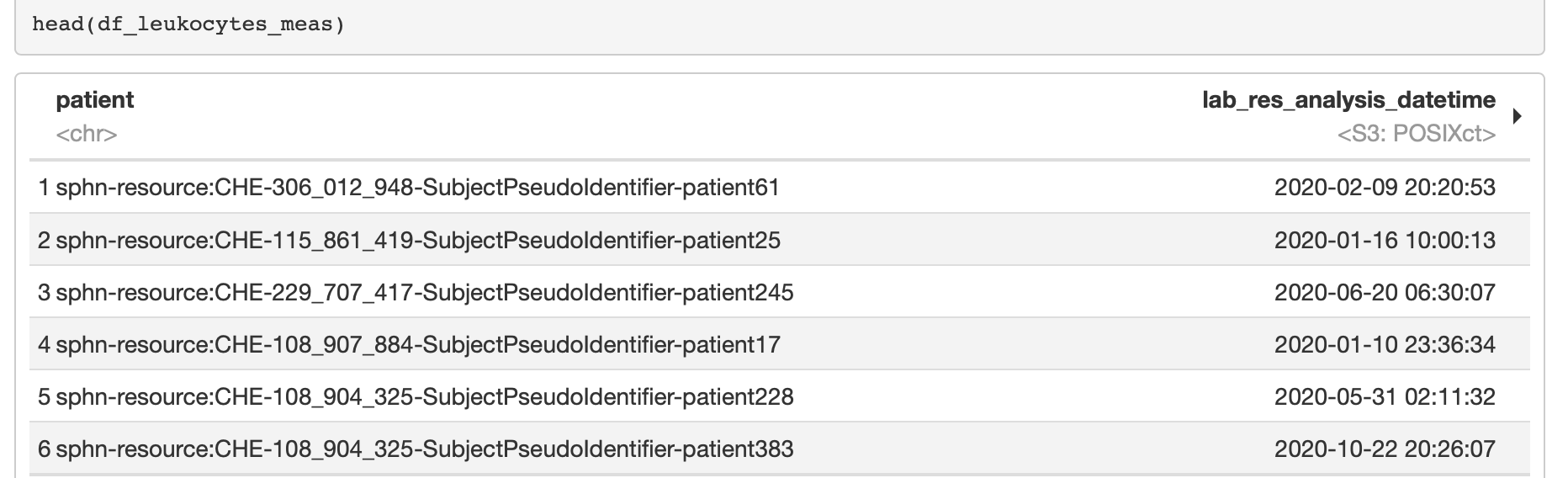
Figure 9: Excerpt of the results following the datatype conversion in R.

Merging the dataframes

Merging the dataframes is done by performing a left (outer) join for dataframes df_pulse_vegetable and df_leukocytes_meas on the patient variable. The resulting dataframe contains all values of the df_pulse_vegetable, and also the matching values of the df_leukocytes_meas.

Python

Left (outer) join is performed in Python using the pandas merge function, as shown in the following code block (see Figure 10 for an excerpt of the results):

# merge the two dataframes on having same patients
df =  pd.merge(df_pulse_vegetable,
               df_leukocytes_meas,
               how='left',
               on='patient')

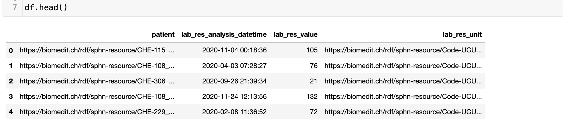
Figure 10: Excerpt of the results following the merging the dataframes in Python.

R

Left (outer) join is performed in R using the left_join function, as shown in the following code block (see Figure 11 for an excerpt of the results):

# left join the two dataframes on having same patients
df =  left_join(df_pulse_vegetable,
            df_leukocytes_meas,
            by=c("patient" = "patient"))

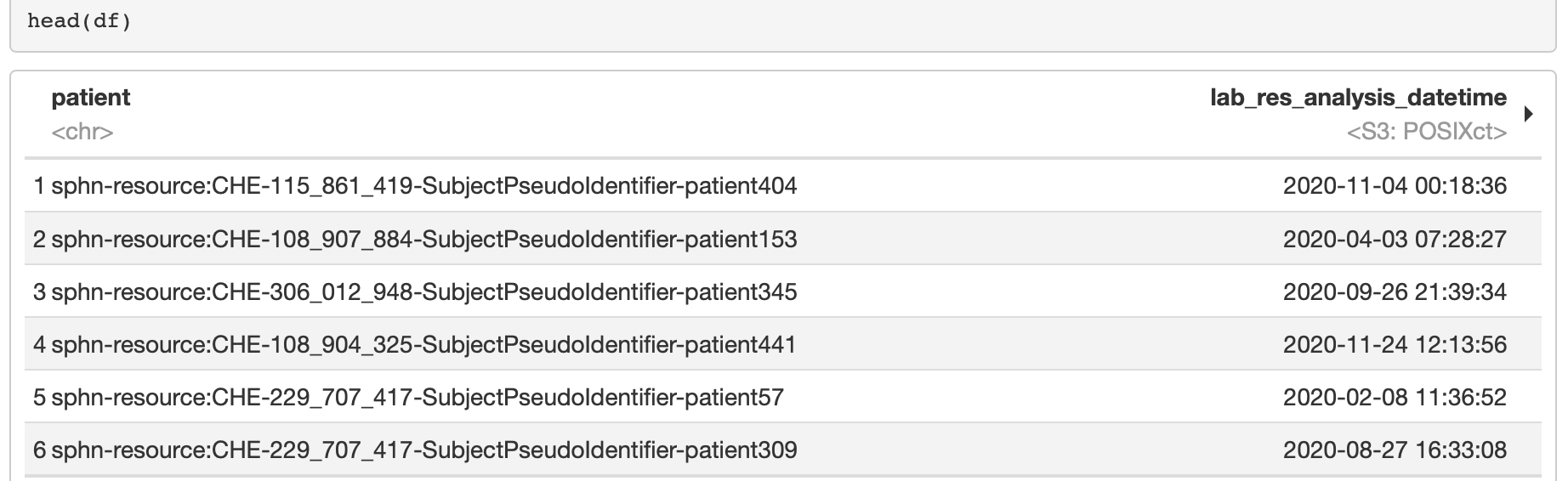
Figure 11: Excerpt of the results following the merging the dataframes in R.

Further Information

For further information, please refer to the following sources:

Python

Python for Data Analysis, 2nd Edition by W. McKinney

Introduction to Data Science in Python by C. Brooks

Python Data Science Handbook by J. VanderPlas

R

R for Data Science by H. Wickham

SPARQL with R in less than 5 minutes