Loading data into GraphDB

This section will go through the various approaches for loading RDF data into GraphDB. For each approach, we will explore how to load the data. Then we will highlight the advantages and disadvantages associated with each approach.

In GraphDB, data are organized within repositories. Each repository is an independent RDF database that can be active independently from other repositories. Operations involving data updates or queries are always directed to a single repository.

There are 3 approaches to loading data into a repository:

GraphDB Workbench
RDF4J API
GraphDB ImportRDF

Depending on the scale of the data, you will have to use one or a combination of approaches.

GraphDB Workbench

The GraphDB Workbench is the web interface of the GraphDB instance (typically accessible via https://localhost:7200). The workbench allows users to create and manage repositories, load and export data, execute SPARQL queries, manage users and perform other operations for administering a GraphDB instance.

You can load RDF data into a repository via the GraphDB Workbench but there are some things to consider.

Advantages

Easy loading of RDF data via the GraphDB Workbench
Can upload files into the Workbench to load data into a repository
Can also load snippets of RDF into a repository

Disadvantages

Only small files are supported (up to 200 MB)
Moderate to slow speed depending on the size of the target repository

Note

The size of 200 MB is not fixed. You can change the permitted file size via the graphdb.workbench.maxUploadSize system property. But this configuration needs to be supplied to GraphDB at runtime using the -Dgraphdb.workbench.maxUploadSize flag. See GraphDB Documentation on Importing local files for more information.

The next section will provide step-by-step instructions on how to load data into a repository using the GraphDB Workbench.

Step 1: Create and configure a repository

First go to the GraphDB Workbench on the browser. You should see a landing page as shown below.

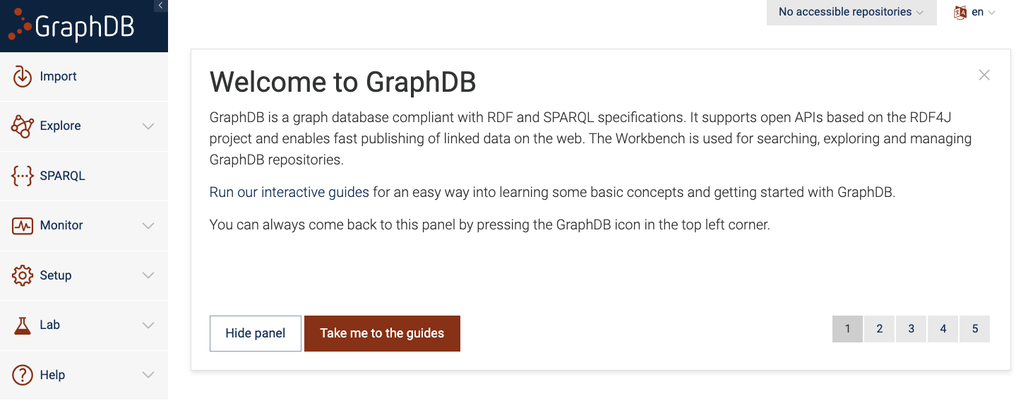
Figure 1: GraphDB Workbench

To create a new repository, click on ‘Create new repository’ button and and select ‘GraphDB Repository’ option. Then you will be shown a page where you can configure your repository.

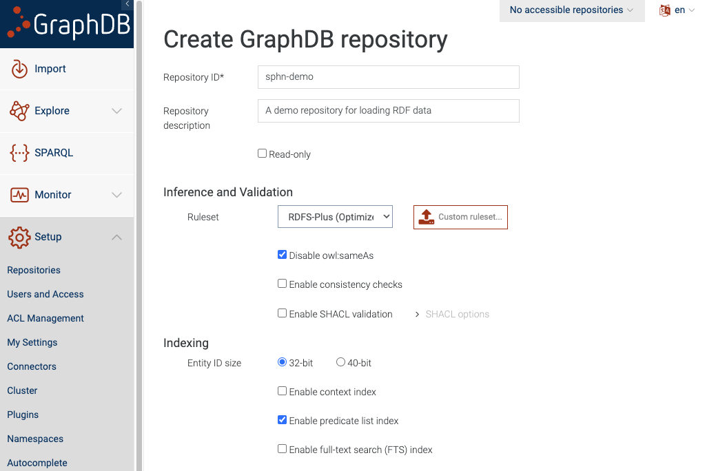
Figure 2: Configure the new repository

Add the name of your repository and then click the ‘Create’ button.

It is perfectly fine to leave the rest of the settings on default. You may want to change them if you have different requirements like specific inference capabilities or adding SHACL validation directly to the repository.

Note

These configurations can only be set at the time of creating the repository. If any of these configurations need to change then you will have to create a new repository with the new configurations.

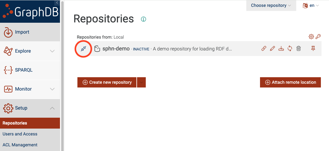
Figure 3: Connect to the repository

Now you will see the sphn-demo as one of the repositories. You can click on the ‘connect’ icon, circled in red, to connect to the repository.

Step 2: Import data

After you are connected to the repository, you can click on the ‘Import’ button from the sidebar. This will give you different options on how to load your data. GraphDB supports a variety of input formats for RDF such as *.ttl, *.rdf, *.n3, *.nt, *.nq, *.trig, *.owl as well as their compressed versions (i.e. gzip or zip).

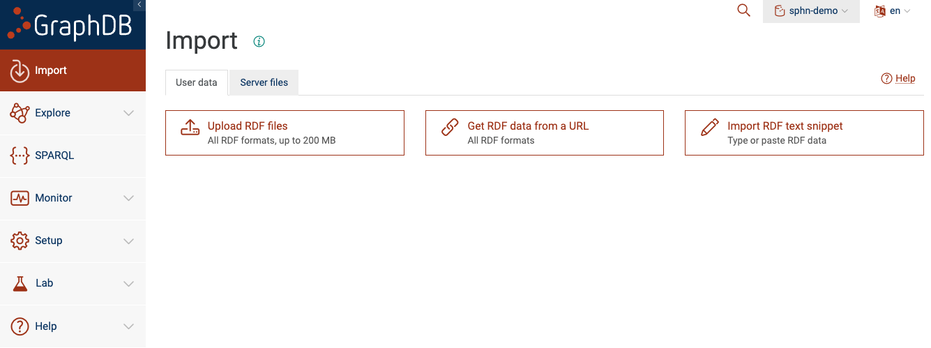
Figure 4: Import data to the repository

You will see that there are two tabs: ‘User data’ and ‘Server files’.

There are four different ways you can load data directly from the GraphDB Workbench:

Upload RDF files
Get RDF data from a URL
Import RDF text snippets
Import from server files

Option A: Upload RDF files

You can click on ‘Upload RDF files’ and select the RDF file (from your local filesystem) that you would like to load into the repository.

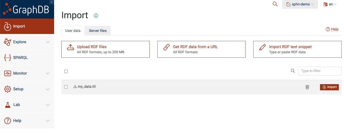
Figure 5: Upload RDF data to the repository

You will see that the uploaded file is now listed as one of the files to import.

Note

This option only supports files that are less than 200 MB in size (by default).

Now you can tick the checkbox for my_data.ttl and click on the ‘Import’ button. You will be presented with a dialog box:

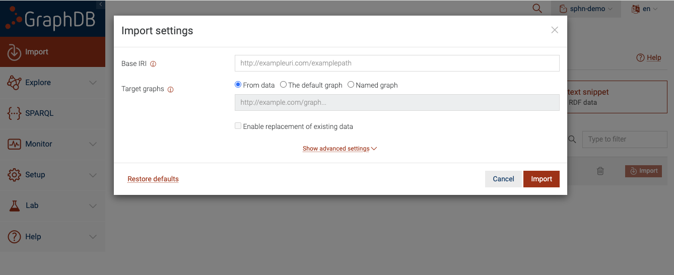
Figure 6: Import RDF data into the repository

It is perfectly fine to leave these settings on default. Once you click ‘Import’, GraphDB will parse the contents of my_data.ttl and load the triples into the sphn-demo repository.

Option B: Get RDF data from a URL

You can also load RDF data into your repository from a file that is located at a URL.

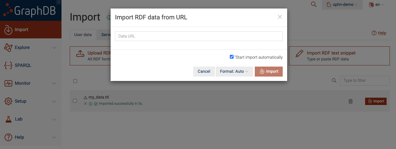
Figure 7: Import RDF data via URL

This approach is useful provided that the RDF data is available via a URL. For the sake of this example, you can use https://git.dcc.sib.swiss/sphn-semantic-framework/sphn-ontology/-/raw/master/rdf_schema/sphn_rdf_schema.ttl.

After you paste the URL and click ‘Import’, GraphDB automatically figures out the incoming data format (based on the content) and loads it into the sphn-demo repository.

Option C: Import RDF text snippets

You can also load snippets of RDF data into your repository.

Figure 8: Import RDF text snippet.

You can paste your RDF triples (in an appropriate format) into the text box and then click ‘Import’. For the sake of an example, you can copy and paste the following text into the text field:

@prefix sphn: <https://biomedit.ch/rdf/sphn-schema/sphn#> .
@prefix snomed: <http://snomed.info/id/> .
@prefix rdf: <http://www.w3.org/1999/02/22-rdf-syntax-ns#> .
@prefix resource: <https://biomedit.ch/rdf/sphn-resource/> .

# types
resource:hospital1-SubjectPseudoIdentifier-anonymous1 rdf:type sphn:SubjectPseudoIdentifier .
resource:hospital1-DataProvider rdf:type sphn:DataProvider .

resource:hospital1-Allergy-allergy1 rdf:type sphn:Allergy .
resource:hospital1-Allergen-peanuts1 rdf:type sphn:Allergen ;
    sphn:hasCode resource:Code-SNOMED-CT-762952008 .
resource:Code-SNOMED-CT-762952008 rdf:type snomed:762952008 .

# relations to the allergy
resource:hospital1-Allergy-allergy1 sphn:hasSubjectPseudoIdentifier resource:hospital1-SubjectPseudoIdentifier-anonymous1 .
resource:hospital1-Allergy-allergy1 sphn:hasDataProvider resource:hospital1-DataProvider .
resource:hospital1-Allergy-allergy1 sphn:hasAllergen resource:hospital1-Allergen-peanuts1 .

After clicking on ‘Import’, GraphDB loads the snippet into the sphn-demo repository.

Option D: Import from server files

If enabled on your GraphDB instance (by the administrator), data in a dedicated folder can be made available to the GraphDB Workbench. Be sure to place your RDF data files directly to this dedicated folder so that it is visible to GraphDB.

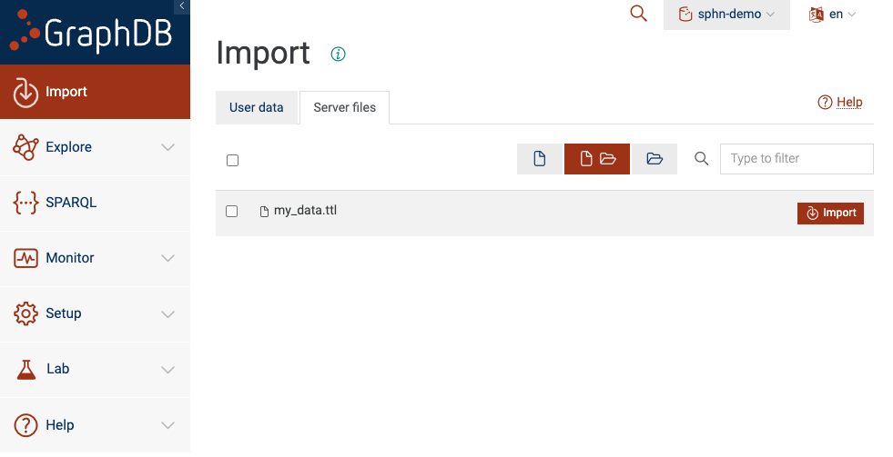
Figure 9: Import Server files

You will see all files and folders placed within the dedicated folder. In this example, we see that my_data.ttl is visible to the GraphDB because it was placed in the dedicated folder. To import the data into your repository, be sure to select the appropriate files and then click ‘Import’.

Note

The exact location of this folder on the filesystem is configurable via the graphdb.workbench.importDirectory system property. See GraphDB Documentation on Importing server files for more information.

Loading into a named graph

You can also load the data into a named graph by defining a unique IRI that corresponds to the named graph. When you click on the ‘Import’ button, you should see a settings dialog with various configuration options.

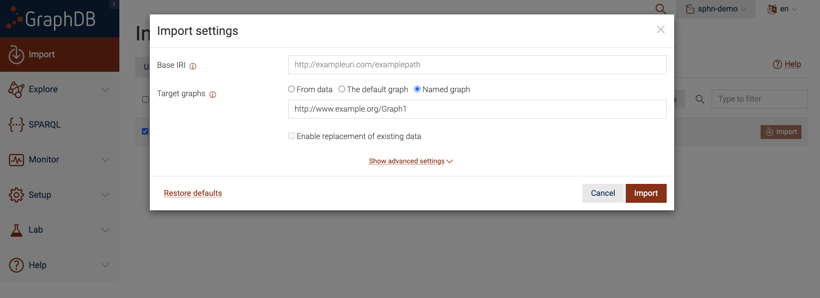
Figure 10: Import Server files to a Named Graph

To ensure that the triples are loaded into a named graph, be sure to click on ‘Named graph’ for the ‘Target graphs’ section and provide an IRI for the named graph. This IRI should be unique for each named graph. In the above figure, we use http://www.example.org/Graph1 as the IRI for our named graph. After which, you can click on ‘Import’ and this should load all triples from my_data.ttl into the named graph instead of the default graph. To load more data into the named graph, be sure to use the exact same IRI to refer to the named graph.

Named graphs are useful for partitioning your graph into different subgraphs, each of which can be identified using its IRI. For more information on Named Graphs see section Named Graphs.

RDF4J API

The RDF4J API is a widely used Java framework for working with RDF data and interacting with triple stores. In the context of GraphDB, the RDF4J API serves as the programmatic interface for managing and interacting with repositories, performing data operations, and executing SPARQL queries. The RDF4J API is particularly useful when you need fine-grained control over data loading and integration with other applications or systems. See GraphDB Documentation on Using GraphDB with the RDF4J API for more information.

Loading RDF data into a GraphDB repository via the RDF4J API often involves making HTTP requests to specific API endpoints. The curl command-line tool is a commonly used utility for sending HTTP requests. But you can make use of any HTTP client.

Advantages

Quite easy to load data into a repository via the API
Easy to automate the process of loading data into a repository
Can be used to load data into a repository in an incremental manner (i.e. delta loads)

Disadvantages

It is not recommended to load billions of triples via the API

We will demonstrate this approach using curl. You can load data into a repository as follows:

curl -X POST -H "Content-Type:application/x-turtle" -T my_data.ttl \
    http://localhost:7200/repositories/sphn-demo/statements

The above curl command is sending an HTTP POST request where:

content type in the request header is set to application/x-turtle
-T option indicates that my_data.ttl file is being uploaded from local to destination
destination URL is http://localhost:7200/repositories/sphn-demo/statements which indicates that the GraphDB is located at http://localhost:7200 and the repository name is sphn-demo.

Note

The repository must exist before this operation is performed.

Tip

You can access the RDF4J API for GraphDB via http://localhost:7200/webapi.

Loading into a named graph

The RDF4J API provides several endpoints to interact with a GraphDB repository. Using the API, you can also load data into a named graph instead of the default graph.

Find all named graphs in a repository

First, lets find out all the named graphs that already exist in a GraphDB repository. You can make use of the http://localhost:7200/repositories/<repository_name>/contexts endpoint that lists all the contexts (or rather named graphs) that exists in the repository.

Using curl you can interact with this endpoint as follows:

curl -X GET --header 'Accept: application/sparql-results+json' \
    'http://localhost:7200/repositories/sphn-demo/contexts'

The above curl command is sending an HTTP GET request where:

the response content type is set to application/sparql-results+json
the endpoint URL is http://localhost:7200/repositories/sphn-demo/contexts

You should see the following response:

{
    "head" : {
        "vars" : [
        "contextID"
        ]
    },
    "results" : {
        "bindings" : [ ]
    }
}

Based on the response we see that there are no named graphs currently in sphn-demo repository.

Load data into a named graph

There are two ways you load data into a named graph via the API. You can make use of either:

http://localhost:7200/repositories/<repository_name>/rdf-graphs/<name_of_named_graph>
http://localhost:7200/repositories/<repository_name>/rdf-graphs/service?graph=<iri_of_named_graph>

You can load data into a named graph using either of the endpoints. The choice depends on how you want to name your named graph.

If you use the first endpoint then you do not have to provide a unique IRI. Instead, you provide the name for the named graph and the unique IRI is prepared automatically based on the repository IRI. For example, lets assume we want to load the triples into a named graph with the name my-new-named-graph-1.

Then you can use http://localhost:7200/repositories/<repository_name>/rdf-graphs/<name_of_named_graph> as follows:

curl -X POST --header 'Content-Type: text/turtle' -T my_data.ttl \
    'http://localhost:7200/repositories/sphn-demo/rdf-graphs/my-new-named-graph-1'

The above curl command is sending an HTTP POST request where:

content type in the request header is set to application/x-turtle
-T option indicates that my_data.ttl file is being uploaded from local to destination
the destination URL is http://localhost:7200/repositories/sphn-demo/rdf-graphs/my-new-named-graph-1 where the repository is sphn-demo and the name of the named graph is my-new-named-graph-1.

One thing to keep in mind is that in this example we do not define a unique IRI for the named graph ourselves. Instead, we just provide a simple name for the named graph and GraphDB automatically makes a unique IRI for the named graph.

We can see this by querying the http://localhost:7200/repositories/<repository_name>/contexts endpoint again:

curl -X GET --header 'Accept: application/sparql-results+json' \
    'http://localhost:7200/repositories/sphn-demo/contexts'

And we get the following response:

{
    "head" : {
        "vars" : [
        "contextID"
        ]
    },
    "results" : {
        "bindings" : [
        {
            "contextID" : {
            "type" : "uri",
            "value" : "http://localhost:7200/repositories/sphn-demo/rdf-graphs/my-new-named-graph-1"
            }
        }
        ]
    }
}

Note how there is now one context (i.e. named graph) with an IRI of http://localhost:7200/repositories/sphn-demo/rdf-graphs/my-new-named-graph-1.

This is fine if we are not opinionated about the IRI for the named graph. But if we do want more control over the IRI of the named graph then we have to make use of the second endpoint (http://localhost:7200/repositories/<repository_name>/rdf-graphs/service?graph=<iri_of_named_graph>) where we are explicitly stating the IRI for the named graph. For example, lets assume we want to load the triples into a named graph with a unique IRI http://www.example.org/my-new-named-graph-1.

curl -X POST --header 'Content-Type: text/turtle' -T my_data.ttl \
    'http://localhost:7200/repositories/sphn-demo/rdf-graphs/service?graph=http%3A%2F%2Fwww.example.org%2Fmy-new-named-graph-1'

The above curl command is sending an HTTP POST request where:

content type in the request header is set to application/x-turtle
-T option indicates that my_data.ttl file is being uploaded from local to destination
the destination URL is http://localhost:7200/repositories/sphn-demo/rdf-graphs/service?graph=http%3A%2F%2Fwww.example.org%2Fmy-new-named-graph-1 where the repository is sphn-demo and the unique IRI of the named graph is http://www.example.org/my-new-named-graph-1

Tip

When providing IRIs as an argument in the URL of API calls, be sure to URL encode the IRIs. In the above example the IRI http://www.example.org/my-new-named-graph-1 is encoded to http%3A%2F%2Fwww.example.org%2Fmy-new-named-graph-1 such that it is safe to be sent as an argument in the request URL.

Now if we query the http://localhost:7200/repositories/<repository_name>/contexts endpoint again:

curl -X GET --header 'Accept: application/sparql-results+json' \
    'http://localhost:7200/repositories/sphn-demo/contexts'

We get the following response:

{
    "head" : {
        "vars" : [
        "contextID"
        ]
    },
    "results" : {
        "bindings" : [
        {
            "contextID" : {
            "type" : "uri",
            "value" : "http://localhost:7200/repositories/sphn-demo/rdf-graphs/my-new-named-graph-1"
            }
        },
        {
            "contextID" : {
            "type" : "uri",
            "value" : "http://www.example.org/my-new-named-graph-1"
            }
        }
        ]
    }
}

Note how there are two named graphs where both have the same name i.e. my-new-named-graph-1 but the IRIs are different. The named graph with IRI http://localhost:7200/repositories/sphn-demo/rdf-graphs/my-new-named-graph-1 was created when we did not care about the exact IRI associated with the named graph. The named graph with IRI http://www.example.org/my-new-named-graph-1 was created when we provided the exact IRI for the named graph as part of the request.

Deleting data from a named graph

To delete all the data that is in a named graph, you can make use of the same endpoint as before. But this time, use the HTTP DELETE method instead of HTTP POST. For example, if we want to delete all the triples in the http://www.example.org/my-new-named-graph-1 named graph:

curl -X DELETE --header 'Accept: application/sparql-results+json' \
    'http://localhost:7200/repositories/sphn-demo/rdf-graphs/service?graph=http%3A%2F%2Fwww.example.org%2Fmy-new-named-graph-1'

The above curl command is sending an HTTP DELETE request where:

the response content type is set to application/sparql-results+json
the destination URL is http://localhost:7200/repositories/sphn-demo/rdf-graphs/service?graph=http%3A%2F%2Fwww.example.org%2Fmy-new-named-graph-1 where the repository is sphn-demo and the IRI of the named graph is http://www.example.org/my-new-named-graph-1

Now if we query the http://localhost:7200/repositories/<repository_name>/contexts endpoint:

curl -X GET --header 'Accept: application/sparql-results+json' \
    'http://localhost:7200/repositories/sphn-demo/contexts'

And we get the following response:

{
    "head" : {
        "vars" : [
        "contextID"
        ]
    },
    "results" : {
        "bindings" : [
        {
            "contextID" : {
            "type" : "uri",
            "value" : "http://localhost:7200/repositories/sphn-demo/rdf-graphs/my-new-named-graph-1"
            }
        }
        ]
    }
}

Note how there is only one named graph instead of two.

GraphDB ImportRDF

Another approach for loading RDF data into a GraphDB repository is ImportRDF, a tool designed for loading large amounts of RDF data. The ImportRDF tool is bundled with the GraphDB distribution and can be found in the bin folder of the GraphDB installation directory. Thus, you do need access to the command line and access to the GraphDB installation to be able run the ImportRDF tool.

Advantages

Fast and performant loading of RDF data into a repository

Disadvantages

The GraphDB instance has to be shutdown before the loading can be performed
ImportRDF writes to an empty repository. Thus, incremental loading (i.e. delta loads) is not possible
Requires a signficant amount of memory, especially when trying to load billions of triples

The ImportRDF tool has two subcommands: load and preload. Depending on the use case, you will have to choose which subcommand is appropriate for loading your data.

ImportRDF load

The load subcommand operates on large amounts of RDF data. It parses and transforms the RDF files into GraphDB images using an algorithm similar to the one used for online loading of data. As the data variety grows, the loading speed starts to decrease. This slowdown becomes apparent when comparing the number of triples parsed at the beginning of the loading process with those parsed at the end.

The main benefit of the load subcommand is that after processing all the data, it also runs inference at the very end. This means that if your use case relies on inference capabilities, then the load subcommand is a more suitable choice.

You can run the load subcommand to load data into an existing repository, provided that this repository is empty. You can also use the --force flag to overwrite the repository.

Alternatively, you can create a new repository by providing a repository configuration - a turtle file that descibes the configurations of the repository in RDF. A template for this repository configuration is as follows:

# Configuration template for a GraphDB repository

@prefix rdfs: <http://www.w3.org/2000/01/rdf-schema#>.
@prefix rep: <http://www.openrdf.org/config/repository#>.
@prefix sr: <http://www.openrdf.org/config/repository/sail#>.
@prefix sail: <http://www.openrdf.org/config/sail#>.
@prefix graphdb: <http://www.ontotext.com/trree/graphdb#>.

[] a rep:Repository ;
    rep:repositoryID "sphn-demo-new" ;
    rdfs:label "A demo repository for loading SPHN data" ;
    rep:repositoryImpl [
    rep:repositoryType "graphdb:SailRepository" ;
    sr:sailImpl [
        sail:sailType "graphdb:Sail" ;

            # ruleset to use
            graphdb:ruleset "rdfsPlus-optimized" ;

            # disable context index(because my data do not uses contexts)
            graphdb:enable-context-index "false" ;

            # indexes to speed up the read queries
            graphdb:enablePredicateList "true" ;
            graphdb:enable-literal-index "true" ;
            graphdb:in-memory-literal-properties "true" ;
    ]
].

The above configuration can be used with the ImportRDF tool to create a new repository called sphn-demo-new and then load all the triples into this repository.

To run the load subcommand:

/opt/graphdb/dist/bin/importrdf load -m parallel -c repository_config.ttl my_data.ttl >& importrdf_load.log

Where:

the loading mode is set to parallel as configured by the --mode flag
the repository configuration repository_config.ttl is provided by the --config-file flag
the input RDF data my_data.ttl is provided as the last argument

The assumption here is that the importrdf tool is located at /opt/graphdb/dist/bin. This location may be different for you depending on where and how the GraphDB instance is installed on your system.

To tweak your loading performance see GraphDB Documentation on ImportRDF - Tuning load.

Tip

It is always advisable to keep track of the logs so that it is easy to investigate loading performance and keep track of when the loading was done and how.

ImportRDF preload

Similar to the load subcommand, the preload operates on large amounts of RDF data, parses and transforms RDF files into GraphDB images. However, it makes use of a different algorithm where the process initially involves parsing all RDF triples in-memory, dividing them into manageable chunks, and then subsequently writing these chunks to disk as multiple GraphDB images. Finally, all these individual chunks are merged into a single GraphDB image. As a consequence of this approach, running the “preload” subcommand requires nearly double the disk space compared to the “load” subcommand and a substantial amount of system memory.

The main benefit of preload subcommand is that it is fast and capable of processing billions of triples efficiently. This is the recommended approach for loading large amounts of data into a GraphDB repository. One thing to keep in mind is that the preload does not perform inference on the data.

Note

When dealing with large amounts of RDF data, it is not practical to expect inference since it adds a great deal of overhead depending on the different rules that apply to the triples. If inference is really desired then an alternative would be to infer and materialize triples ahead of time such that these inferred triples are part of your input RDF data.

You can run the preload subcommand to load data into an existing repository, provided that this repository is empty. You can also use the --force flag to overwrite the repository.

Alternatively, you can create a new repository by providing a repository configuration - a turtle file that descibes the configurations of the repository in RDF. A template for this repository configuration is as follows:

# Configuration template for a GraphDB repository

@prefix rdfs: <http://www.w3.org/2000/01/rdf-schema#>.
@prefix rep: <http://www.openrdf.org/config/repository#>.
@prefix sr: <http://www.openrdf.org/config/repository/sail#>.
@prefix sail: <http://www.openrdf.org/config/sail#>.
@prefix graphdb: <http://www.ontotext.com/trree/graphdb#>.

[] a rep:Repository ;
    rep:repositoryID "sphn-demo-new" ;
    rdfs:label "A demo repository for loading SPHN data" ;
    rep:repositoryImpl [
    rep:repositoryType "graphdb:SailRepository" ;
    sr:sailImpl [
        sail:sailType "graphdb:Sail" ;

            # ruleset to use
            graphdb:ruleset "empty" ;

            # disable context index(because my data do not uses contexts)
            graphdb:enable-context-index "false" ;

            # indexes to speed up the read queries
            graphdb:enablePredicateList "true" ;
            graphdb:enable-literal-index "true" ;
            graphdb:in-memory-literal-properties "true" ;
    ]
].

The above configuration can be used with the ImportRDF tool to create a new repository called sphn-demo-new and then load all the triples into this repository.

To run the preload subcommand:

/opt/graphdb/dist/bin/importrdf preload --config-file repository_config.ttl my_data.ttl >& importrdf_preload.log

Where:

the repository configuration repository_config.ttl is provided by the --config-file flag
the input RDF data my_data.ttl is provided as the last argument

The preload automatically determines various load specfic parameters like iterator cache size, number of chunks and number of RDF parsers. You can configure this manually to tweak your loading performance. See the GraphDB Documentation on ImportRDF - Tuning preload for more information.

Tip

It is always advisable to keep track of the logs so that it is easy to investigate loading performance and keep track of when the loading was done and how.

Loading into a named graph

Due to the offline nature of data loading with the ImportRDF tool, it is not possible to specify which named graph to load the data to. But there is a workaround to this limitation.

When working with RDF data, there are different ways how RDF statements can be represented. The most common is an RDF triple where each statement is a combination of a subject, predicate, and object. These triples can be serialized into a file and the format is N-Triples (*.nt).

# RDF statement as a triple
resource:CHE-115_861_419-DataProviderInstitute-AdministrativeGender-00295d34-b264-43d5-990e-b9ee9478c1d4 rdf:type sphn:AdministrativeGender .

In the above snippet, the triple represents an RDF statement that exists in the default graph.

There is also another style of representation called N-Quads where each statement is represented as a combination of subject, predicate, object, and the graph to which the statement belongs to. N-Quads can be serialized into a file and the corresponding file format is N-Quads (*.nq).

# RDF statement as an N-Quad
resource:CHE-115_861_419-DataProviderInstitute-AdministrativeGender-00295d34-b264-43d5-990e-b9ee9478c1d4 rdf:type sphn:AdministrativeGender <http://www.example.org/my-new-named-graph-1> .

In the above snippet, the N-Quad represents an RDF statement that exists in a named graph identified by a unique IRI http://www.example.org/my-new-named-graph-1.

Thus, you could take your RDF triples and convert them to N-Quads such that you deliberately assign the named graph to which each triple belongs to. And then use this N-Quads representation of your data as input for the ImportRDF tool. This ensures that your triples are loaded into the appropraite named graph in your repository.

Note

Monitoring resources while importing data

System resources, such as memory and CPU consumption, can be monitored via the GraphDB Workbench. You can navigate to “Monitor” and then click on “System” button.

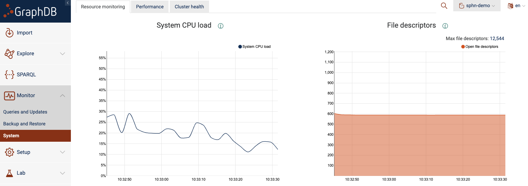
Figure 11: Resource monitoring.

This can be helpful to debug issues with excessive resource consumption, especially when importing large datasets.